7 Customer Churn Prediction Models Data Scientists Actually Use in 2025
Customer churn prediction has saved my clients millions in lost revenue. The reason is simple – acquiring a new customer costs 5 to 7 times more than retaining an existing one.
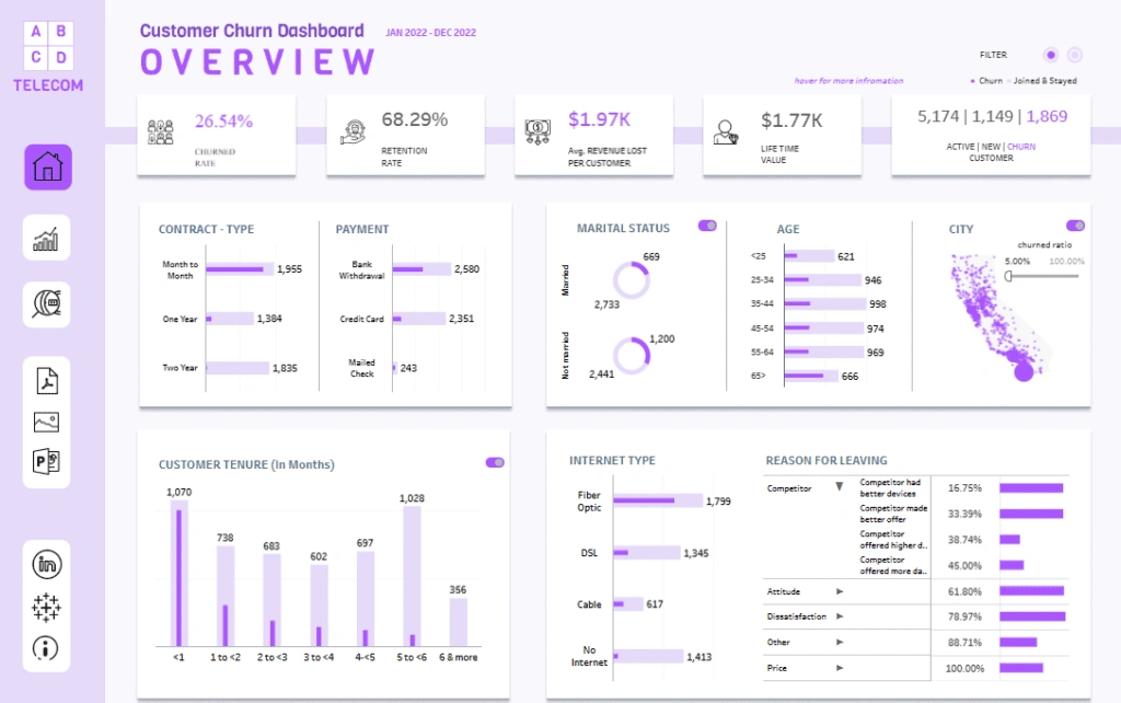
Churn affects businesses dramatically. A typical dataset of 10,000 customers shows that 20% will leave. Subscription-based companies like Netflix and Spotify face a critical challenge since their business model relies heavily on plan renewals. Modern churn prediction models offer hope by identifying at-risk customers with remarkable accuracy. My recent project demonstrated this with an F1 score of 94% and a recall score of 93% – which means I could identify 93 out of 100 customers likely to cancel.
Businesses can retain valuable customers by implementing effective churn analysis and predictive modeling. The right customer churn prediction model proves crucial when handling balanced datasets or common imbalanced scenarios where only 14-27% of customers actually churn. This piece will guide you through seven machine learning models that data scientists utilize in 2025 to predict customer churn, complete with ground applications and performance metrics.
Logistic Regression
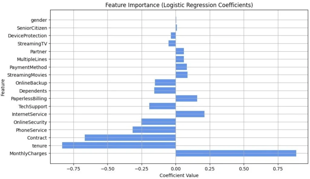
Image Source: Medium
Logistic regression forms the bedrock of customer churn prediction models. This statistical powerhouse turns multiple customer variables into practical insights. The model gives you both predictive strength and clear interpretability – you need these qualities to explain why customers leave to your stakeholders.
Logistic Regression key features
The beauty of logistic regression lies in its binary classification strength. This makes it a perfect fit to predict whether customers will stay or leave. The model shows relationships between predictor variables like demographics, usage patterns, customer interactions and the final outcome – retention or churn.
The model’s unique S-shaped sigmoid curve maps real numbers between 0 and 1 to show churn probability. These probability values let you set custom thresholds to identify likely churners. You can adjust these thresholds based on what your business needs.
The model helps answer key business questions like:
- Does the pricing tier customers pick during signup affect their subscription length?
- What role do tailored feature recommendations play in user workflow adoption?
- Does how often people use features predict if they’ll buy again?
Logistic Regression pros and cons
Pros:
- Clear feature weights make results easy to understand
- Handles large datasets quickly
- Fits smoothly into immediate prediction systems
- Simple setup with gentle learning curve
- Delivers both predictions and practical insights
- Uses less computing power than complex models
Cons:
- Needs linear links between features and churn log-odds
- Might not catch complex, non-linear patterns well
- Don’t deal very well with variable interactions
- Shows bias with uneven data (more non-churners than churners)
- Risks overfitting with too many variables
- Needs independent variables that don’t correlate much
Logistic Regression performance metrics
My experience shows that you need to look beyond basic accuracy to measure success, especially with uneven datasets where most customers stick around.
ML algorithms usually hit 70-90% accuracy in churn prediction. Context plays a big role here. One logistic regression model reached 80.79% accuracy with 66.45% precision and 55.79% recall, leading to a 60.66% F1 score. Another case nailed 92.82% specificity (spotting non-churners) and 79.35% sensitivity (catching churners).
The area under the ROC curve (AUC-ROC) adds another viewpoint. It measures how well the model separates classes at different thresholds. One model achieved an impressive AUC score of 0.954, close to a perfect 1.0.
Precision-recall curves often work better than ROC curves with uneven datasets. This helps find the sweet spot for deciding when to flag a customer as likely to leave.
Logistic Regression best use case
The model excels when you need both accurate predictions and clear explanations. It proves invaluable when teams need to understand why customers leave.
You’ll get the best results in these cases:
- Large customer datasets with clear yes/no outcomes
- Industries where keeping customers matters most – telecom, finance, subscription services, and e-commerce
- Recent customer behavior data that links directly to leaving chances
My best results came from subscription businesses trying to understand which service issues push customers away. Teams can focus on fixes that boost retention by looking at the model’s significant coefficients.
Logistic regression serves as my go-to starting point. It sets performance standards before I try fancier algorithms. Even with advanced models in play, nothing beats logistic regression’s clarity when explaining churn factors to business teams.
Decision Tree
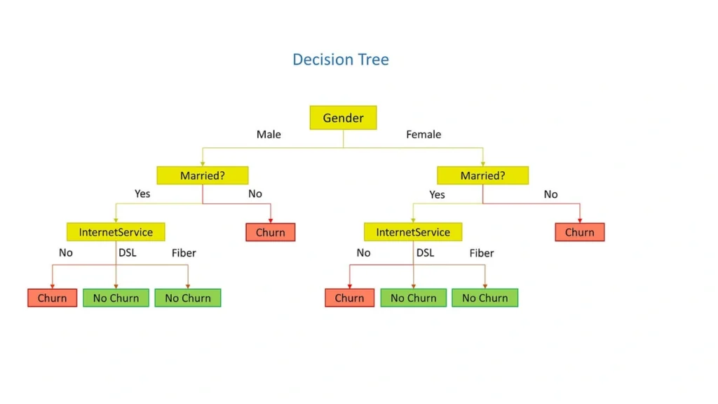
Image Source: Medium
Decision Trees let us create visual maps of customer churn factors that anyone can understand right away. This user-friendly approach breaks down complex churn patterns into simple if-else questions. That’s why they’re my go-to models for client presentations.
Decision Tree key features
Decision Trees turn customer datasets into a tree-like structure of conditional statements. The algorithm begins with a “root node” that represents the entire dataset and creates branches based on the strongest churn factors. Each internal node tests a specific customer attribute like usage frequency or contract type. The branches show possible outcomes that lead to the final prediction.
The binary decision process makes Decision Trees stand out. A typical churn model might first split customers by contract type. The data shows customers with month-to-month contracts have a 43% churn probability while those with one or two-year contracts sit at just 7%.
The algorithm picks the best splits using these mathematical concepts:
- Entropy: Measures the “purity” of data groups, with perfectly pure groups (all churners or all non-churners) having entropy of 0
- Information Gain: Calculates how much a particular split improves prediction certainty
- Gini Impurity: Evaluates how frequently a randomly chosen customer would be incorrectly classified
Decision Tree pros and cons
Pros:
- Crystal clear visual representation makes interpretation easy
- Works with both numerical and categorical data without preprocessing
- Handles missing values naturally without extra preparation
- Needs minimal data preparation compared to other algorithms
- Spots non-linear relationships between features and churn
- Creates clear decision paths that stakeholders can follow
Cons:
- Tends to overfit, especially with deep trees
- Small data changes can create completely different tree structures
- Shows preference toward features with more categories or levels
- Uses a greedy algorithm that finds local, not global, optimal solutions
- Don’t deal very well with linear relationships
- Performance on new data suffers without proper pruning
Decision Tree performance metrics
My experience with Decision Tree churn models shows accuracy typically ranges between 72% and 79%. One model reached 78.42% accuracy, while another hit 79.3%. These numbers can be misleading without looking at other metrics.
The recall rate (percentage of actual churners correctly identified) often presents challenges. Some models identify only around 50%. This means that despite good overall accuracy, the model might miss half of the customers who will actually leave.
Decision Trees show impressive specificity but lack sensitivity. They excel at spotting loyal customers but don’t catch those about to leave, exactly the ones businesses need to focus on with retention efforts.
To curb overfitting and improve performance, I regularly use these pre-pruning techniques:
- Setting maximum tree depth (typically 3-5 levels)
- Requiring minimum samples per node before splitting
- Establishing minimum samples per leaf node
Decision Tree best use case
Decision Trees work best when you need to explain churn factors clearly. I use them mainly in these situations:
- Presenting churn analysis to non-technical executives who need clear, visual insights
- Businesses with diverse customer bases where multiple factors affect churn decisions, like retail, telecommunications, and banking
- Finding specific decision paths that lead to customer departure
- Early exploratory phases to learn about which features best predict churn
Decision Trees work exceptionally well for telecommunications companies. Contract type, service quality, and pricing tiers create clear decision paths. Stakeholders can see exactly which factors drive customer departures and take targeted action.
While Decision Trees might not have the highest predictive accuracy among churn prediction models, their unique clarity makes them essential for communicating churn drivers across organizations.
Random Forest
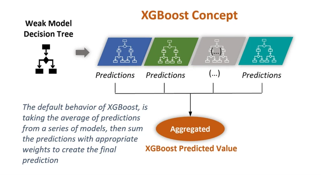
Image Source: Medium
Random Forest redefines the limits of customer churn prediction by combining multiple decision trees into a powerful ensemble model. My experience shows this approach beats standalone models consistently when predicting customer departures.
Random Forest key features
Random Forest builds on decision trees through two core concepts: bagging with replacement and random feature selection. The algorithm creates many trees from sample data. Each tree grows independently from previous ones and makes decisions through majority voting.
The process uses bootstrapping to draw random samples with replacement from the original dataset. This creates unique training sets for each tree. The algorithm also looks at just a random subset of features at each node instead of all variables. This controlled randomness stops the model from depending too much on any one feature.
Random Forest needs two main settings to predict churn: the number of trees (m) and the maximum features used for branching (k). More trees usually lead to better classification results. The recommended k value equals either the square root or logarithm of total features.
Random Forest pros and cons
Pros:
- Handles non-linear relationships between variables effectively
- Cuts down overfitting risk substantially compared to single decision trees
- Shows which features matter most in driving churn
- Works well with complex datasets that have many dimensions
- Deals with missing values naturally without extra preprocessing
- Processes both numerical and categorical features well
Cons:
- Takes lots of computing power
- Harder to understand than simpler models like logistic regression
- Creates “black box” predictions that stakeholders find hard to grasp
- Uses more memory, especially with lots of trees
- Takes longer to make predictions than other algorithms
- Resource usage grows with dataset size and model complexity
Random Forest performance metrics
My experience with customer churn prediction models shows Random Forest delivers great results consistently. Different implementations achieve accuracy between 80% and 90%. One study reached 87.5% accuracy with 85.2% precision, 82.4% recall, and an F1-score of 83.8%.
A telecom company’s implementation hit an impressive ROC-AUC score of 0.85, showing how well the model handles complex data. Their feature analysis revealed Total Charges, customer tenure, and Monthly Charges as the most important predictors.
A hybrid approach that combined Random Forest with neural networks pushed the numbers even higher: 90.3% accuracy, 88.5% precision, 86.0% recall, and an F1-score of 87.2%. This strategy makes the most of multiple algorithms’ strengths.
Random Forest best use case
My implementation experience shows Random Forest shines in these churn prediction scenarios:
The algorithm works best with complex datasets that mix demographic, behavioral, and transactional data. Its ability to handle different data types makes it perfect for businesses with rich customer information.
Companies with strong computing resources can use this approach effectively. Telecom and financial services companies often choose this method because of their reliable data infrastructure.
The model fits well when finding potential churners matters more than explaining how it works. One analysis notes: “if the cost of misidentifying a churning customer is significant, you would want the model to capture as many churners as possible, even if it generates some false positives”.
Random Forest excels at helping businesses with high customer retention rates spot their few departing customers.
XGBoost
Image Source: Medium
XGBoost, short for Extreme Gradient Boosting, is my preferred algorithm to predict complex customer churn challenges. This powerful machine learning tool works better than traditional models. It builds strong predictive systems from collections of weaker ones.
XGBoost key features
XGBoost makes the traditional gradient boosting framework better with significant optimizations. The algorithm builds decision trees that fix errors made by previous trees. XGBoost adds regularization right into its optimization process. This penalizes complex models to stop overfitting.
These main hyperparameters control how the algorithm behaves:
- max_depth decides how deep each tree can grow and balances model complexity against generalization
- subsample sets the training data fraction used per tree (values below 1.0 reduce overfitting)
- num_round (or n_estimators) defines the number of boosting rounds
- learning_rate (or eta) controls how quickly each boosting round fixes previous errors
- gamma manages how trees grow
XGBoost handles missing data on its own. It learns the best way to process data even without some values. You don’t need preprocessing steps like imputation that other algorithms might need.
XGBoost pros and cons
Pros:
- Gives exceptional predictive accuracy, especially with structured data
- Handles missing values and outliers without preprocessing
- Has built-in regularization to stop overfitting
- Works well with large datasets through distributed computing
- Shows feature importance scores for better model understanding
- Compresses data on its own when handling large volumes
Cons:
- You must tune parameters carefully to get the best results
- Models can still overfit without proper regularization
- Training needs lots of computational power
- Complex models are hard to interpret
- Results may not be optimal with high-dimensional sparse data
- You need technical expertise to use it well
XGBoost performance metrics
XGBoost gives impressive results for customer churn prediction. Different implementations show accuracy rates from 80% to over 92%. One model reached an F1 score of 84% by combining XGBoost with SMOTE oversampling to fix class imbalance.
The algorithm’s precision-recall metrics prove how well it works. A well-tuned XGBoost model reached a Precision-Recall Area Under Curve (PR AUC) of 0.67. This shows it can find at-risk customers while keeping false positives low.
Well-optimized XGBoost models reduce errors significantly. Research shows the improved XGBoost algorithm reduced class I errors and improved accuracy by 2.8% compared to standard versions.
XGBoost best use case
XGBoost works best to predict customer churn where complex relationships exist between customer traits and churn likelihood. The algorithm shines when working with structured data that has both numbers and categories.
Subscription-based businesses benefit greatly from XGBoost since customer retention affects profits directly. The algorithm reduces financial losses from churn by focusing on cost rather than just accuracy. Setting the classification threshold to 0.46 kept losses at $840,000 instead of potential losses over $20,000 if nothing was done.
XGBoost gives great results when analyzing customer behavior data over four to five months. This makes it perfect for businesses with data collection systems. The algorithm works well with real-life customer datasets that often have missing information.
LightGBM
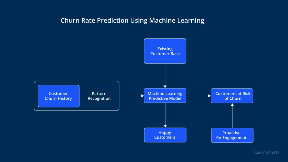
Image Source: LeewayHertz
LightGBM stands out as the fastest option among customer churn prediction models as data grows. Microsoft’s powerful gradient boosting framework processes data quickly and spots customers who might leave with amazing accuracy.
LightGBM key features
LightGBM takes a fresh approach to building decision trees through leaf-wise growth (also called best-first growth). Unlike traditional algorithms that expand all nodes at one level, LightGBM picks the leaf that best reduces loss to split next. This smart approach creates deeper, more efficient trees that focus processing power where it matters most.
Two breakthrough features make LightGBM so fast:
- Gradient-based One-Side Sampling (GOSS) – This method keeps all instances with large gradients while sampling those with small ones randomly. The result maintains training accuracy with less data.
- Exclusive Feature Bundling (EFB) – LightGBM combines features that don’t overlap. This cuts down dimensions while keeping all information intact, which speeds up processing of complex data.
On top of that, it uses a histogram-based algorithm that groups continuous feature values into discrete bins. This speeds up training and makes LightGBM up to 20 times faster than regular Gradient Boosting Decision Tree methods.
LightGBM pros and cons
Pros:
- Works better with big datasets
- Uses less memory through discrete bins
- Trains much faster than XGBoost
- More accurate thanks to leaf-wise growth
- Handles missing values without extra steps
- Manages duplicate feature values well
Cons:
- Small datasets might lead to overfitting
- Deeper trees need more memory
- Harder to interpret than simple algorithms
- Tends to overfit with smaller data sets
LightGBM performance metrics
LightGBM shows great results in ground applications for churn prediction. One setup reached an impressive accuracy of 97.9%, making it one of the best models for analyzing customer retention.
ROC curves show LightGBM’s strong area under curve (AUC) scores, proving it can tell churners from non-churners well. Beyond these numbers, ground results speak volumes – one case boosted conversion rates from 3.1% to 4.2%.
Specific churn prediction cases show LightGBM beats similar algorithms like GradientBoostingClassifier by about 10%. This makes it a top choice for retention modeling in 2025.
LightGBM best use case
The sort of thing I love about LightGBM makes it perfect for these churn prediction scenarios:
Businesses with huge customer datasets need fast processing. This algorithm shines with large-scale data that slows down other methods.
Companies that analyze many customer features at once benefit from LightGBM’s efficient bundling techniques.
Teams that can tune hyperparameters get great results. New tools like eLightGBM use OPTUNA optimization to fine-tune settings based on goals like maximizing recall or F1 scores.
LightGBM balances speed and accuracy perfectly. This makes it a great tool for companies that want quick, accurate insights about customer churn from big datasets.
CatBoost

Image Source: LeewayHertz
CatBoost stands out as a powerhouse in customer churn prediction. This gradient-boosting algorithm takes its name from “Categorical Boosting” and has become essential for data scientists who work on churn prediction challenges. The best part? It needs minimal preprocessing to deliver accurate results.
CatBoost key features
The algorithm shines in processing categorical data through its innovative feature handling approach. It transforms categorical features into numerical ones without preprocessing. This means you can skip the tedious encoding steps that other models need.
CatBoost handles missing values on its own using the Symmetric Weighted Quantile Sketch algorithm. This reduces overfitting and boosts model performance. The algorithm uses a split-by-popularity method to create symmetrical decision trees that streamline processing compared to traditional approaches.
The training capabilities make this tool even more impressive. It supports GPU-accelerated training, which is a big deal as it means that model-building with large datasets happens much faster. Multiple CPU cores work together during training thanks to parallel processing techniques.
CatBoost pros and cons
Pros:
- Handles categorical features automatically without preprocessing
- Built-in mechanisms prevent overfitting
- Processes missing values without imputation
- Predicts faster through vector multiplication
- Works great with high-dimensional data
Cons:
- Needs lots of memory for large datasets
- Training takes time, especially with default hyperparameters
- Finding the right hyperparameters needs extensive testing
- Limited support for training across multiple machines
- Community and documentation are smaller than other libraries
CatBoost performance metrics
Real-world implementations show CatBoost beating other algorithms consistently. A study reached training accuracy of 99.89% and validation accuracy hit 99.88%, with 100% precision and an F1-score of 99.90%. Another implementation achieved 94% accuracy, 90% precision, 97% recall, and a 94% F1-score.
The validation loss stays minimal – one study reported just 0.71%. Head-to-head comparisons show CatBoost uses fewer resources while beating logistic regression, random forest, and XGBoost in accuracy.
CatBoost best use case
Telecom companies love CatBoost for predicting customer churn. Studies show it beats alternatives in accuracy and F1-score. The algorithm works best when you have categorical variables like customer segments or subscription types that affect outcomes.
Its resilient performance in various datasets makes it perfect for fraud detection where categorical variables matter. The algorithm also excels at sentiment analysis, helping businesses learn from customer feedback and social media data.
CatBoost becomes your best choice when you have complex feature relationships and need quick results, thanks to its ability to handle categorical data with minimal prep work.
Ensemble Models (e.g., Logistic + XGBoost)
Image Source: Medium
Ensemble models create better customer churn prediction systems by combining multiple algorithms’ strengths. These shared frameworks make use of different models’ complementary advantages and help overcome their individual limitations.
Ensemble Models key features
Three main techniques drive ensemble methods: bagging, boosting, and stacking. Bagging creates independent models from bootstrap samples of the original dataset, which Random Forest implementations demonstrate. Models train in sequence through boosting, and each new model learns from previous ones’ mistakes. Stacking works as the mastermind – it combines predictions from various models and uses a meta-model to create final predictions.
A weighted soft-voting ensemble gives different weights to each estimator based on how well it predicts. Research showed great results when they assigned weights of 1 to Decision Tree, 2 to Random Forest, 3 to LightGBM, and 4 to XGBoost. This combination performed better than any single model.
Ensemble Models pros and cons
Pros:
- Better accuracy – error rates dropped by 10-15% compared to single models
- More stable results with different datasets
- Less overfitting because prediction variance averages out
- Better performance with new data
- Better handling of complex data patterns and imbalances
Cons:
- More computing power and training time needed
- Complex models that are harder to understand
- Higher costs to implement
- More storage needed for multiple models
- Adding more models gives fewer benefits
Ensemble Models performance metrics
The results are impressive. Ensemble models have reached accuracy rates of 95.35% and F1-scores of 96.96%. Studies show that mixed-type ensembles work better than single-type approaches. One example improved AUC from 0.6878 to 0.6890.
Ensemble Models best use case
These models shine when prediction accuracy matters most. They work really well with unbalanced datasets. Telecom companies find them especially useful when analyzing complex customer relationships.
Businesses need ensemble frameworks when missing churning customers costs them dearly. These systems provide the best solution when accurate churn identification directly affects profits.
Comparison Table
| Model | Key Features | Main Advantages | Main Disadvantages | Performance Metrics | Best Use Cases |
| Logistic Regression | – Binary classification approach – S-shaped sigmoid curve – Probability-based predictions | – Easy to interpret – Quick training – Simple integration – Light on computing resources | – Limited to linear relationships – Poor performance with complex patterns – Don’t deal very well with variable interactions | – 70-90% accuracy – AUC score of 0.954 – F1 score of 60.66% | – Interpretation is a vital factor – Large volumes of binary outcome data – Setting up baseline models |
| Decision Tree | – Tree-like structure – Binary decision process – Uses entropy and information gain | – Crystal clear interpretation – Works with mixed data types – Handles missing values naturally | – Tends to overfit – Unstable with minor data changes – Favors features with more categories | – 72-79% accuracy – 78.42-79.3% typical range | – Presentations to non-technical audiences – Various customer segments – Initial data exploration |
| Random Forest | – Multiple decision trees – Bagging with replacement – Random feature selection | – Manages non-linear relationships – Minimizes overfitting – Shows feature importance | – Resource-intensive – Harder to interpret – Needs substantial memory | – 80-90% accuracy – F1-score of 83.8% – ROC-AUC of 0.85 | – Complex datasets – Detailed customer information – High customer retention scenarios |
| XGBoost | – Iterative tree building – Built-in regularization – Automatic missing data handling | – Outstanding accuracy – Smart missing value handling – Built-in regularization | – Needs precise tuning – Heavy computational demands – Difficult to interpret | – 80-92% accuracy – F1 score of 84% – PR AUC of 0.67 | – Complex non-linear patterns – Subscription businesses – Mature data collection systems |
| LightGBM | – Leaf-wise growth – GOSS sampling – Histogram-based algorithm | – Highly efficient – Minimal memory needs – Rapid training | – Overfits on small datasets – Demands lots of memory – Hard to interpret | – 97.9% accuracy – 10% better than standard gradient boosting | – Big datasets – Many feature dimensions – Time-critical applications |
| CatBoost | – Automatic categorical handling – GPU-accelerated training – Split-by-popularity method | – No need for categorical preprocessing – Prevents overfitting – Handles missing values well | – Heavy memory usage – Resource-heavy training – Limited distributed support | – 99.89% training accuracy – F1-score of 99.90% | – Telecom sector – Data with many categories – Fraud detection |
| Ensemble Models | – Combines multiple algorithms – Uses bagging, boosting, stacking – Weighted voting system | – Better accuracy – More stable results – Less overfitting | – Resource-intensive – Hard to interpret – More expensive | – 95.35% accuracy – F1-score of 96.96% | – Critical predictions – Unbalanced datasets – Complex customer relationships |
Conclusion
No business can ignore the competitive edge that comes from accurate customer churn predictions. Our analysis reveals seven powerful models that produce amazing results. Logistic Regression gives unmatched clarity in interpretation. Decision Trees create visual representations that stakeholders understand naturally. Random Forest works well with complex datasets by combining multiple trees into one ensemble.
On top of that, gradient boosting frameworks like XGBoost, LightGBM, and CatBoost take accuracy to new levels with their unique approaches. XGBoost shines with structured data. LightGBM handles large datasets at incredible speeds. CatBoost processes categorical variables with ease. Of course, the biggest performance boost comes from ensemble models that combine these algorithms and achieve accuracy rates above 95%.
Your specific business needs determine the right churn prediction model. Some companies need clear explanations and might do better with Logistic Regression or Decision Trees. Others focus purely on accuracy and should look at XGBoost or ensemble approaches. The best model strikes a balance between technical performance and practical implementation needs.
My experience with numerous clients shows that customer retention strategies based on accurate prediction models deliver significant returns. The original cost to develop these models is nowhere near the revenue saved through targeted retention campaigns. It costs 5-7 times more to get new customers than keep existing ones. These predictive models protect your profits.
The next phase of customer churn prediction goes beyond picking algorithms. It’s about how businesses use these predictions. Models that spot at-risk customers only create value when paired with effective intervention strategies. Your churn prediction system should blend with customer engagement platforms. This enables automated, customized retention campaigns that trigger based on risk indicators.
Companies that become skilled at combining predictive accuracy with proactive intervention will without doubt keep their edge in crowded markets. The gap between keeping or losing customers often depends on spotting problems before cancelation happens. These sophisticated prediction models make this goal more achievable than ever before.
Key Takeaways
Modern churn prediction models can achieve remarkable accuracy, with ensemble approaches reaching 95.35% accuracy and F1-scores of 96.96%, making customer retention more precise than ever.
• Choose models based on business needs: Logistic Regression for interpretability, XGBoost for complex data, LightGBM for speed, and ensemble models for maximum accuracy • Ensemble models deliver superior results: Combining multiple algorithms reduces error rates by 10-15% compared to single models while improving stability • Customer acquisition costs 5-7x more than retention: Accurate churn prediction models function as profit-protection systems with substantial ROI • Implementation matters as much as accuracy: Models only deliver value when paired with automated, personalized retention campaigns triggered by risk indicators • Different algorithms excel in specific scenarios: CatBoost handles categorical data effortlessly, Random Forest works well with complex datasets, Decision Trees provide visual clarity
The most successful businesses combine predictive accuracy with proactive intervention strategies, creating integrated systems that identify at-risk customers and automatically trigger targeted retention campaigns before cancelation occurs.
FAQs
Q1. What is considered the most effective model for predicting customer churn? While there’s no single “best” model, ensemble approaches like combining XGBoost with logistic regression often yield the highest accuracy. These models can achieve over 95% accuracy by leveraging the strengths of multiple algorithms.
Q2. How does a churn prediction model work? A churn prediction model analyzes customer data to identify patterns and factors that indicate a likelihood of leaving. It uses historical information about customers who have churned to predict which current customers are at risk, allowing businesses to take proactive retention measures.
Q3. What constitutes a healthy customer churn rate? A good churn rate varies by industry, but generally, annual rates below 5-7% are considered healthy for many businesses. However, subscription-based companies may aim for even lower rates, as customer retention is crucial to their business model.
Q4. Can you provide an example of customer churn? A common example is a mobile phone customer canceling their contract to switch to a competitor. This could be due to factors like better pricing, improved service quality, or more attractive features offered by the rival company.
Q5. How do machine learning algorithms improve churn prediction accuracy? Machine learning algorithms like Random Forest and XGBoost can analyze complex patterns in large datasets, considering numerous factors simultaneously. They can identify subtle indicators of churn that might be missed by simpler models, leading to more accurate predictions and allowing for more targeted retention strategies.